Introduction

Despite their reputation for being (human) error-prone, spreadsheets are indispensable tools in many areas of financial modeling. In recent years, Microsoft Excel has introduced new features that could benefit many users. This post aims to introduce these modern features using a walkthrough of building a tool for interpolating numbers, a common need in financial modeling work.

Spreadsheets: good and bad

Spreadsheets have an unfortunate reputation for being “bad” or “misused”. Bugs or human errors are usually considered commonplace in spreadsheets. Yet, despite this shortcoming, spreadsheets are widely used or sometimes even indispensable, particularly in financial modeling; this implies they must meet particular user needs.

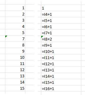
If we look at spreadsheets through the lens of computer science, their most significant weakness lies in their almost constant violation of the DRY principle of programming: Don’t Repeat Yourself. Many formulas are created by copying and pasting cells; this is a necessary feature as it makes it easy for non-programmers to build a spreadsheet quickly. However, it is akin to programming without writing any functions and instead always always copying and pasting code. This pattern inevitably significantly increases the risk of human errors. Excel has a feature that highlights potential cell formula errors based on any formula dissimilarity compared to the formula in surrounding cells. However, in my experience, this has never been of much help in detecting errors in practical usage. The picture below shows what this looks like on a PC. The little green triangle indicates to the user that the cell may contain mistakes in its formula. As can be seen in the picture, when the formula is revealed (through the “show” function on the “formula” ribbon bar in Excel), there is a “+2” instead of “+1”, which Excel correctly guessed is a mistake.

The need for a quick-and-dirty tool is not only due to the need to cater to non-programmers but also for many use cases, including rapid prototyping, quick estimate, discussion of model logic with coworkers or other parties such as auditors, etc. To replace all spreadsheets with program code would be akin to replacing all weakly-typed programming languages like Python and JavaScript with strongly-typed programming languages like Haskell: the end product will have fewer bugs at the expense of taking much longer to deploy, assuming that it even arrives at all, since it would be nearly impossible to find the people with the skill set to do the work!

In contrast, spreadsheets’ greatest strength lies in their ability to provide instantaneous feedback, which is particularly important in financial modeling as most users rely on how the actual numbers look to get a sense of the overall picture. This aspect is highly similar to the read-eval-print loop (REPL) workflow in programming or live reload in webpage design, where the programmer or the designer relies on getting continuous and immediate feedback while working and making changes. This work style also has a similar parallel in the programming world, where scriptlike dynamic languages like Python and JavaScript are invaluable for their ease of experimentation, contributing to higher productivity in certain situations.

A new era in spreadsheets

As with most problems in the real world, great solutions tend to involve some compromise combined with some innovations, usually brought about by the evolution of technology. In recent years, Microsoft Excel has contributed significantly to addressing the general weaknesses of spreadsheets by introducing:

1. New formulas that help readability. Most of these are the new formulas with a plural name, such as SUMIFS. The most important ones are LET and IFS, which I will cover later in this post.
2. Dynamic arrays. You may have noticed that Excel has automatically converted some of your existing spreadsheet formulas to have an “@” sign in your formulas, or you might have seen the “#SPILL!” error and wondered what that is. These are clues to the new functionality in Excel: dynamic arrays. Dynamic arrays differ from the existing array formulas (with “{“ and “}” signs, activated by typing the shift key with the enter key at the same time after entering the formula) mainly in the sense that they can adapt to variable-sized data; however, this fundamental distinction alone makes a massive difference as it allows Excel to follow the DRY principle much closer.
3. LAMBDA. LAMBDA allows the user to define their own function, which looks like VBA or Office Script (JavaScript) User Defined Functions (UDFs) but all calculations in a LAMBDA function are Excel functions. Hence, all calculations can be easily reproduced and checked in Excel. In addition, it also means that the calculations in a LAMBDA will be done in “Excel style”, i.e., declarative form, which ensures that it is easier to read compared to most UDFs which are written in a imperative style. Finally, a LAMBDA offers one crucial advantage over VBA UDFs: safety. VBA code can access all of Windows’ system APIs, making it a security threat; this is why Office on the cloud (Excel on the web) only allows Office Script add-ins and not VBA add-ins. As more workflows move to the cloud, sharing Office documents, including Excel files, will become more common, and LAMBDA will make it safe for everyone to share their custom-built functions.

I will introduce all of the above by building a LAMBDA function in Excel that can calculate cubic spline interpolations and extrapolations. Specifically, the complete calculations will be done in two different ways: first in a spreadsheet using dynamic arrays and other formulas and then again in a LAMBDA function that can be saved and reused in other spreadsheets. Note that LAMBDA functions are saved as “defined names” in Excel (see LAMBDA formula below); to bring them over to other spreadsheets, move or copy any sheet from the source spreadsheet to your new spreadsheet.

If you have experience with Power BI in Excel, you may have noticed that Power BI can also help address some of the DRY issues in financial modeling; for example, the tables in the Power Pivot Data Model can replace many repeated VLOOKUPs with a single RELATED. There is some overlap here between data analysis features and financial modeling features. I will not cover these in this post but may visit this in future posts.

Resources and important notes

For the rest of this post, refer to the Excel spreadsheet on this public GitHub repository under my account.

You need to download the file from the GitHub repository to view it. However, you need Microsoft 365 to view and edit the file. In addition, the modern features discussed in this post may or may not be available in your Microsoft Office, depending on your software license. If you have trouble using that file, you can open and view it online on the cloud without any software installed or license.

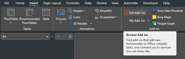
For the rest of this post, I recommmend that you install Microsoft’s new Excel Labs add-in by going to “Get Add-ins” in your Excel’s “Insert” ribbon bar.

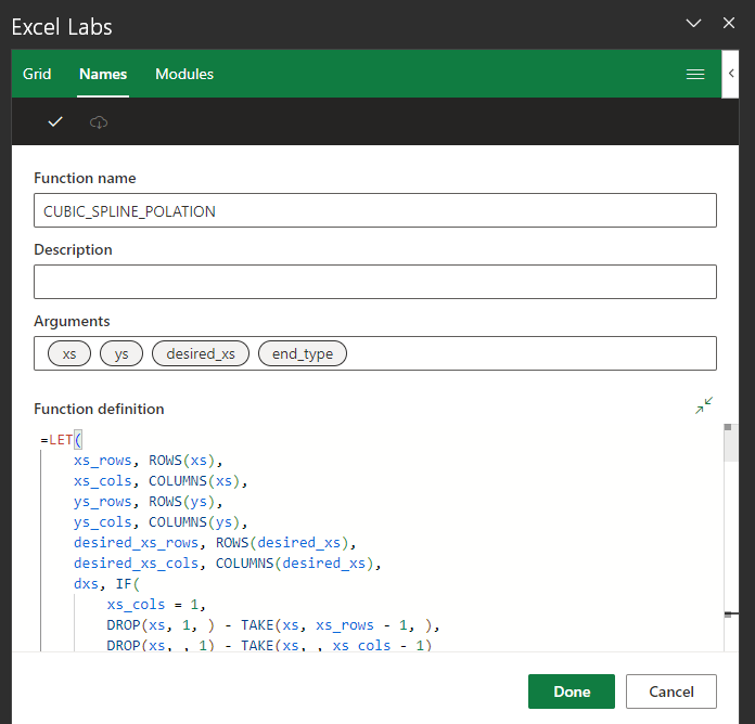
The Excel Labs add-in will highlight and format your formula as shown below, making it much easier for you to work, especially when dealing with LAMBDAs.

Before we proceed, you can try out the “dark mode” by tapping or clicking on the icon on the upper right of your screen. You can turn it off by tapping or clicking again. You might find some formulas easier to read in “dark mode”.

Cubic spline interpolation

Motivation for use

In financial modeling work, there are often situations with gaps in data points where the exact values for the points in between are not particularly important for the task or purpose at hand as long as the numbers are reasonable, i.e., lie “smoothly” between the available data points. A typical example is in market data, where not all points (e.g. tenors) are liquid. A simple but robust and reliable approach to interpolate or extrapolate would be to use a class of curves called cubic splines; see picture below. Since cubic splines are third-order polynomials, they can be smooth enough to fit various shapes yet stiff enough not to be unstable or run wild. Since the starting and ending points do not have anywhere else to “smooth into”, there are alternative variations of cubic spline interpolation methods, depending on the desired restrictions on the two extreme endpoints. The “not-a-knot” and “natural” versions are popular among these alternatives. This post will cover only these two versions.

Necessary formulas for implementation

The formulas for the natural and the not-a-knot versions are available on Wikipedia. The following is a summary that we will use to implement our calculations.

Assume that we have \(n + 1\) points:

\[(x_0,y_0),(x_1,y_1),\ldots ,(x_n,y_n)\]

where

\[x_0\leq x_1\leq x_2\leq x_3\leq \ldots \leq x_n\]

In between any two points, we join them with a cubic equation for a total of \(n\) equations. Between any two consecutive points \(x_i\) and \(x_{i-1}\) we have:

\[q_i(x) = (1-t_i(x))y_{i-1}+t_i(x)y_i+t_i(x)(1-t_i(x))((1-t_i(x))a_i+t_i(x)b_i)\]

where

\[t_i(x)=\frac{x-x_{i-1}}{x_i-x_{i-1}}\] \[a_i=k_{i-1}(x_i-x_{i-1})-(y_i-y_{i-1})\] \[b_i=-k_i(x_i-x_{i-1})+(y_i-y_{i-1})\]

To find all the \(a_i\) s and \(b_i\) s, first we need to find the \(k_i\) s. They are given by the equation:

\[\begin{pmatrix} k_0 \\ \vdots \\ k_n \end{pmatrix}=F^{-1} \times \vec{g}\]

where \(F\) is a square matrix of size \((n+1)\times (n+1)\) and \(\vec{g}\) is a column vector with \((n+1)\) rows. The only differences between natural spline and not-a-knot spline are in the first and last rows of \(F\) and \(\vec{g}\). The other rows are:

\[F = \begin{bmatrix} ? & ? & ? & 0 & 0 & \cdots & 0 & 0 & 0 & 0 & 0 \\ \frac{1}{\Delta x_1} & (\frac{2}{\Delta x_1}+\frac{2}{\Delta x_2}) & \frac{1}{\Delta x_2} & 0 & 0 & \cdots & 0 & 0 & 0 & 0 & 0 \\ 0 & \frac{1}{\Delta x_2} & (\frac{2}{\Delta x_2}+\frac{2}{\Delta x_3}) & \frac{1}{\Delta x_3} & 0 & \cdots & 0 & 0 & 0 & 0 & 0 \\ \cdots & \cdots & \cdots & \cdots & \cdots & \cdots & \cdots & \cdots & \cdots & \cdots & \cdots \\ 0 & 0 & 0 & 0 & 0 & \cdots & 0 & \frac{1}{\Delta x_{n-2}} & (\frac{2}{\Delta x_{n-2}}+\frac{2}{\Delta x_{n-1}}) & \frac{1}{\Delta x_{n-1}} & 0 \\ 0 & 0 & 0 & 0 & 0 & \cdots & 0 & 0 & \frac{1}{\Delta x_{n-1}} & (\frac{2}{\Delta x_{n-1}}+\frac{2}{\Delta x_n}) & \frac{1}{\Delta x_n} \\ 0 & 0 & 0 & 0 & 0 & \cdots & 0 & 0 & ? & ? & ? \\ \end{bmatrix}\] \[\vec{g} = \begin{bmatrix} ? \\ 3(\frac{\Delta y_1}{\Delta x_1^2}+\frac{\Delta y_2}{\Delta x_2^2}) \\ 3(\frac{\Delta y_2}{\Delta x_2^2}+\frac{\Delta y_3}{\Delta x_3^2}) \\ \cdots \\ 3(\frac{\Delta y_{n-2}}{\Delta x_{n-2}^2}+\frac{\Delta y_{n-1}}{\Delta x_{n-1}^2}) \\ 3(\frac{\Delta y_{n-1}}{\Delta x_{n-1}^2}+\frac{\Delta y_n}{\Delta x_n^2}) \\ ? \\ \end{bmatrix}\]

where

\[\Delta x_i=x_i-x_{i-1}\] \[\Delta y_i=y_i-y_{i-1}\]

For natural spline, the question marks above are:

\[F = \begin{bmatrix} \frac{2}{\Delta x_1} & \frac{1}{\Delta x_1} & 0 & 0 & 0 & \cdots & 0 & 0 & 0 & 0 & 0 \\ \cdots & \cdots & \cdots & \cdots & \cdots & \cdots & \cdots & \cdots & \cdots & \cdots & \cdots \\ 0 & 0 & 0 & 0 & 0 & \cdots & 0 & 0 & 0 & \frac{1}{\Delta x_n} & \frac{2}{\Delta x_n} \\ \end{bmatrix}\] \[\vec{g} = \begin{bmatrix} 3\frac{\Delta y_1}{\Delta x_1^2} \\ \cdots \\ 3\frac{\Delta y_n}{\Delta x_n^2} \\ \end{bmatrix}\]

For not-a-knot spline, the question marks above are:

\[F = \begin{bmatrix} \frac{1}{\Delta x_1^2} & (\frac{1}{\Delta x_1^2}-\frac{1}{\Delta x_2^2}) & -\frac{1}{\Delta x_2^2} & 0 & 0 & \cdots & 0 & 0 & 0 & 0 & 0 \\ \cdots & \cdots & \cdots & \cdots & \cdots & \cdots & \cdots & \cdots & \cdots & \cdots & \cdots \\ 0 & 0 & 0 & 0 & 0 & \cdots & 0 & 0 & \frac{1}{\Delta x_{n-1}^2} & (\frac{1}{\Delta x_{n-1}^2}-\frac{1}{\Delta x_n^2}) & -\frac{1}{\Delta x_n^2} \\ \end{bmatrix}\] \[\vec{g} = \begin{bmatrix} 2(\frac{\Delta y_1}{\Delta x_1^3}-\frac{\Delta y_2}{\Delta x_2^3}) \\ \cdots \\ 2(\frac{\Delta y_{n-1}}{\Delta x_{n-1}^3}-\frac{\Delta y_n}{\Delta x_n^3}) \\ \end{bmatrix}\]

Spreadsheet calculations

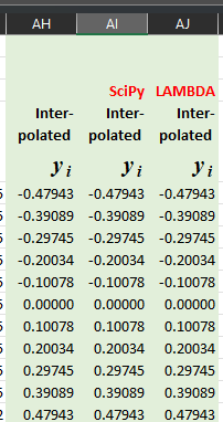
We will first implement the calculations in a sheet. Refer to the sheet “Natural Cubic Spline” in our demo file. The other sheet “Not-a-knot Cubic Spline” is the same except for a few parts in the matrix \(F\) and the column vector \(\vec{g}\), as described earlier. In terms of the overall structure of the sheet, first, pay attention to the final results below. The leftmost column contains the results calculated by this sheet, followed by the numbers calculated by SciPy (a Python library) in the middle column. Finally, the results calculated by our LAMBDA (described below) are in the rightmost column. All three results are independent, and they all agree.

Dynamic arrays

Next, let us start with the inputs, as shown in the picture below. The inputs are directly keyed in by the user in the labeled section “Raw Inputs”. “Original points” refer to the \(x_i\) s and \(y_i\) s of our formulas described earlier, while “For interpolation” are \(x\) values for which we wish to find the interpolated \(y\) values. The section to the right labeled “Dynamic array format” does not perform any numerical calculations but performs an important role in activating dynamic arrays.

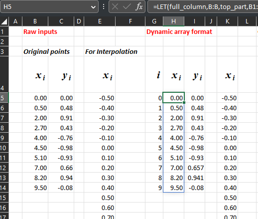
There are three crucial observations here that will immediately show you why dynamic arrays significantly help us follow the DRY principle:

1. A blue rectangle surrounds the dynamic array, even though the user only selected the first cell of the dynamic array. Try to key in more inputs or delete some values in the “Raw Inputs” section. You will notice that the blue rectangle expands or shrinks automatically depending on the data size you entered in “Raw inputs”!
2. There are no “{“ and “}” symbols surrounding the formula in the formula bar, which means that the formula is not the “classical” static array. The picture below shows that, unlike the classical static array, we do not need to refer to our dynamic array using explicit cell ranges in subsequent formulas. Instead, we only need to attach a “#” after the first cell.
3. The picture below shows that certain modern functions like TAKE and DROP are used. These functions perform array operations on dynamic arrays or ranges and behave similarly to functions you may have seen or used in array-based languages or libraries such as MATLAB or Numpy in Python. Hence, we can write formulas that operate on a natural unit of calculation (arrays) instead of individual cells (which are related but cannot be processed together easily as an atomic unit in classical formulas).

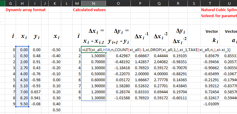
LET

As you may have noticed in the picture above, I have used a function called LET. This powerful new function greatly helps make formulas much more readable by giving names to parts of our calculations. For example, instead of

= A1 + B1

we could now write

= LET(MoneyFromDad, A1,
      MoneyfromMom, B1,
      MoneyFromDad + MoneyFromMom)

this is so easy to read that I find no way to explain any further here. Notice that we can use this function to make our formulas self-documenting by choosing meaningful names.

One point worth mentioning here is that, in addition to making our formulas look more readable, LET can also make our calculations run faster by not repeating portions of our calculations, i.e., portions of calculations that are shared by different calculations can be refactored into a common piece and named inside a LET function. The “classical” approach to do this is to put that common piece of calculation in a separate portion of the spreadsheet, which makes the spreadsheet more crowded and usually more difficult to read.

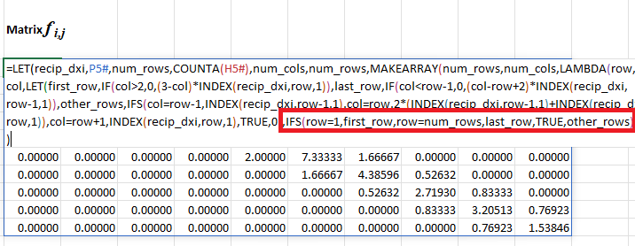
IFS

Similar to LET, the IFS function is also a syntactic sugar, i.e., it does not allow you to do something new that you could not do before. However, just like LET, it has the potential to make your formulas much more readable. You may have had plenty of experience counting brackets in formulas like “=IF(.., ,, IF(…, IF(,…)))”. Such nested IFs is a common pattern in spreadsheets. By switching to writing in IFS like in the picture below, your (coworkers’) nightmares (of reading deeply nested IF functions) are finally over.

Important performance considerations for LET and IFS (and LAMBDAs)

Unfortunately, both IFS and LET do not use lazy (i.e., short-circuit) evaluation: they evaluate all input terms, even terms that are not used and do not contain any volatile function or any UDF with side effects (e.g., write to file). For example:

= LET(X, AVERAGE(SEQUENCE(1000000, 100000, 0, 1)),  
      Y, 0,  
      Y  
  )

and

= IFS(TRUE, 0,  
      FALSE, AVERAGE(SEQUENCE(1000000, 100000, 0, 1))  
      )

and

= LAMBDA(X, Y, Y + 1)    
    (AVERAGE(SEQUENCE(1000000, 100000, 0, 1)), 0)  

will each result in an out-of-memory message, wheareas:

= IF(TRUE, 0,  
     AVERAGE(SEQUENCE(1000000, 100000, 0, 1))  
    )

will work without any issue and give the correct answer of 0.

Hopefully, Microsoft will fix this in the future.

• Thanks to Matt Tarler (@mtarler) on Microsoft Tech Community for pointing out this issue on IFS.

LAMBDA formula

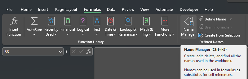
LAMBDA is precisely as its name suggests: an anonymous function. However, like in programming languages that support anonymous functions, an Excel LALMBDA can also be assigned to a named item. Specifically, it can be attached to a named range, as shown in the picture below.

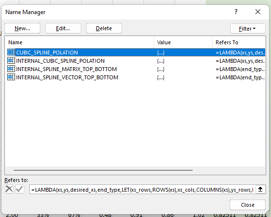
You can bring up the dialog box above by visiting the Name Manager in your Formulas ribbon bar, as shown in the picture below.

There is a limit to the number of characters in the formula of a LAMBDA that you can enter into Excel. Fortunately, a named LAMBDA can call another named LAMBDA. Hence, I have broken down my LAMBDA into pieces. First, I start with a wrapper function that checks that the inputs are valid, and if the inputs are column vectors, the wrapper function will transpose them into row vectors before passing them to the function INTERNAL_CUBIC_SPLINE_POLATION and also transpose the output from INTERNAL_CUBIC_SPLINE_POLATION into a column vector before returning it as the final result. I have used helper functions like ISOMITTED to help check the inputs.

=LET(
    xs_rows, ROWS(xs),
    xs_cols, COLUMNS(xs),
    ys_rows, ROWS(ys),
    ys_cols, COLUMNS(ys),
    desired_xs_rows, ROWS(desired_xs),
    desired_xs_cols, COLUMNS(desired_xs),
    dxs, IF(
        xs_cols = 1,
        DROP(xs, 1, ) - TAKE(xs, xs_rows - 1, ),
        DROP(xs, , 1) - TAKE(xs, , xs_cols - 1)
    ),
    IFS(
        ISOMITTED(xs),
        "Missing argument xs",
        ISOMITTED(ys),
        "Missing argument ys",
        ISOMITTED(desired_xs),
        "Missing argument desired_xs",
        ISOMITTED(end_type),
        "Missing argument end_type",
        AND(xs_rows > 1, xs_cols > 1),
        "Argument xs is a matrix, expecting a vector",
        AND(ys_rows > 1, ys_cols > 1),
        "Argument ys is a matrix, expecting a vector",
        AND(desired_xs_rows > 1, desired_xs_cols > 1),
        "Argument desired_xs is a matrix, expecting a vector",
        xs_rows + xs_cols < 4,
        "Argument xs is too small, need to be a vector with at least 3 elements",
        ys_rows + ys_cols < 4,
        "Argument ys is too small, need to be a vector with at least 3 elements",
        XOR(xs_rows = 1, ys_rows = 1),
        "Arguments xs and ys must be both column vectors or both row vectors, not mixed",
        xs_rows + xs_cols <> ys_rows + ys_cols,
        "Argument vectors xs and ys must both have the same length",
        AND(XOR(xs_rows = 1, desired_xs_rows = 1), desired_xs_rows + desired_xs_cols > 2),
        "Arguments xs and desired xs must be both column vectors or both row vectors, not a mix",
        AND(end_type <> 0, end_type <> 1),
        "Argument end_type must be either 0 for Natural or 1 for Not-a-Knot, no other values permitted",
        OR(dxs < 0),
        "Argument xs must be in increasing order",
        TRUE,
        IF(
            xs_cols = 1,
            INTERNAL_CUBIC_SPLINE_POLATION(xs, ys, desired_xs, end_type),
            TRANSPOSE(
                INTERNAL_CUBIC_SPLINE_POLATION(
                    TRANSPOSE(xs),
                    TRANSPOSE(ys),
                    TRANSPOSE(desired_xs),
                    end_type
                )
            )
        )
    )
)

Next, look at what is inside the INTERNAL_CUBIC_SPLINE_POLATION function, which expects row vectors as inputs and returns a row vector as output. It calculates the matrix \(F\) and the vector \(\vec{g}\) using the functions MAKEARRAY and VSTACK. Then, it calculates the \(k_i\) s and then the \(a_i\) s and \(b_i\) s. Finally, it uses XMATCH on desired_xs to pick the matching \(a_i\) s and \(b_i\) s to calculate the final interpolated \(y\) s.

=LET(
    n, ROWS(xs) - 1,
    dxs, DROP(xs, 1, ) - TAKE(xs, n, ),
    dys, DROP(ys, 1, ) - TAKE(ys, n, ),
    recip_dxs, 1 / dxs,
    recip_dxs_sq, recip_dxs * recip_dxs,
    dy_recip_dxs_sq, dys * recip_dxs_sq,
    matrix_f, MAKEARRAY(
        n + 1,
        n + 1,
        LAMBDA(row, col,
            LET(
                other_rows, IFS(
                    col = row - 1,
                    INDEX(recip_dxs, row - 1, 1),
                    col = row,
                    2 * (INDEX(recip_dxs, row - 1, 1) + INDEX(recip_dxs, row, 1)),
                    col = row + 1,
                    INDEX(recip_dxs, row, 1),
                    TRUE,
                    0
                ),
                IF(
                    OR(row = 1, row = n + 1),
                    INTERNAL_SPLINE_MATRIX_TOP_BOTTOM(end_type, row, col, recip_dxs, recip_dxs_sq),
                    other_rows
                )
            )
        )
    ),
    yi_over_xi2_times3, dy_recip_dxs_sq * 3,
    vec_g_top, INTERNAL_SPLINE_VECTOR_TOP_BOTTOM(end_type, 1, recip_dxs, dy_recip_dxs_sq),
    vec_g_bottom, INTERNAL_SPLINE_VECTOR_TOP_BOTTOM(end_type, n + 1, recip_dxs, dy_recip_dxs_sq),
    vector_g, VSTACK(
        vec_g_top,
        DROP(yi_over_xi2_times3, 1, ) + TAKE(yi_over_xi2_times3, n - 1, ),
        vec_g_bottom
    ),
    ks, MMULT(MINVERSE(matrix_f), vector_g),
    as, TAKE(ks, n, ) * dxs - dys,
    bs, -DROP(ks, 1, ) * dxs + dys,
    min_xi, INDEX(xs, 1, 1),
    max_xi, INDEX(xs, n + 1, 1),
    calc_idxs, IFS(
        desired_xs < min_xi,
        1,
        desired_xs >= max_xi,
        n,
        TRUE,
        XMATCH(desired_xs, xs, -1, 2)
    ),
    lower_xs, INDEX(xs, calc_idxs, 1),
    upper_xs, INDEX(xs, calc_idxs + 1, 1),
    txs, (desired_xs - lower_xs) / (upper_xs - lower_xs),
    one_minus_txs, 1 - txs,
    lower_ys, INDEX(ys, calc_idxs, 1),
    upper_ys, INDEX(ys, calc_idxs + 1, 1),
    ais, INDEX(as, calc_idxs, 1),
    bis, INDEX(bs, calc_idxs, 1),
    one_minus_txs * lower_ys + txs * upper_ys +
        txs * one_minus_txs * (one_minus_txs * ais + txs * bis)
)

The function INTERNAL_CUBIC_SPLINE_POLATION relies on two other helper functions, as shown below.

The function INTERNAL_SPLINE_MATRIX_TOP_BOTTOM calculates the top and bottom rows of matrix \(F\), which varies depending on whether the desired spline type is natural or not-a-knot.

=IF(
    end_type = 0,
    LET(
        i, IF(row = 1, 1, row - 1),
        IFS(
            row = col,
            2 * INDEX(recip_dxs, i, 1),
            OR(col = row + 1, col = row - 1),
            INDEX(recip_dxs, i, 1),
            TRUE,
            0
        )
    ),
    LET(
        c_start, IF(row = 1, 1, row - 2),
        recip1, INDEX(recip_dxs_sq, c_start, 1),
        recip2, INDEX(recip_dxs_sq, c_start + 1, 1),
        IFS(
            col = c_start,
            recip1,
            col = c_start + 1,
            recip1 - recip2,
            col = c_start + 2,
            -recip2,
            TRUE,
            0
        )
    )
)

The function INTERNAL_SPLINE_VECTOR_TOP_BOTTOM calculates the top and bottom rows of vector \(\vec{g}\), which varies depending on whether the desired spline type is natural or not-a-knot.

=IF(
    end_type = 0,
    LET(i, IF(row = 1, 1, row - 1), 3 * INDEX(dys_recip_dxs_sq, i, 1)),
    LET(
        c_start, IF(row = 1, 1, row - 2),
        recip1, INDEX(dys_recip_dxs_sq, c_start, 1) * INDEX(recip_dxs, c_start, 1),
        recip2, INDEX(dys_recip_dxs_sq, c_start + 1, 1) * INDEX(recip_dxs, c_start + 1, 1),
        2 * (recip1 - recip2)
    )
)

As seen above, my LAMBDA does essentially the same calculations as my spreadsheet, except that all the interim results are not shown, and only the final result is returned. This approach is appropriate when we wish to focus on our model rather than nitty-gritty details like the internals of cubic spline interpolation, which has no implications for our work or business as long as it works correctly.

Unfortunately, currently debugging support for LAMBDA is practically non-existent, i.e., no logging, breakpoints, stepping through code, etc. If you have used PowerQuery, this will seem familiar to you.

Validation using SciPy

Validation by SciPy is straightforward using the code shown below. After running this program in a terminal, copy and paste the outputs into our Excel file.

import numpy as np
from scipy.interpolate import CubicSpline
import matplotlib.pyplot as plt
x = [0, 0.5, 2, 2.7, 4, 4.5, 5.1, 7, 8.2, 9.5]
y = np.sin(x)
cs = CubicSpline(x, y, bc_type="not-a-knot")
xs = np.arange(-0.5, 9.6, 0.1)
print("Original x points:")
print(x)
print("Interpolation x points:")
print(xs)
print("Interpolated y points:")
for x in cs(xs):
    print(x)

Future posts

We have only scratched the surface of the new possibilities offered by these modern Excel features. You may already be wondering about questions like:

1. Can a LAMBDA be defined inside a LAMBDA? If so, what are the scope rules of the variables?
2. Can a LAMBDA be called recursively?
3. Can another LAMBDA be passed in as the argument of a LAMBDA?

I plan to share more in future posts. In the meantime, you can read more on all these exciting new productivity enhancements in Excel on Microsoft’s website, such as in this link.

---

(◕‿◕) Please share if you found this post useful: